Classifying Shakespeare with Networks 🍿

All of Shakespeare’s plays, in network form

William Shakespeare is one of our most recognizable and lauded playwrights. With a writing career that spans 36 (easily attributable) plays, an interesting aspect of his work is that these plays can be split up into well defined categories: comedies, tragedies, and histories. Comedies have happy endings and are uplifting, where the main characters overcome some obstacle. Tragedies generally end with the death of a flawed main character. However, how can we formalize the difference between comedies and tragedies? This is what we’ll tackle in this article, but we won’t do it in the way you might expect.

My research (see: cameronraymond.me) focuses on networks and how the connections between us shape our world. While plenty of people have analyzed the dialogue of Shakespeare’s plays, far fewer have bothered to look at the differences in how characters relate to each other. Comedy’s and tragedies are very different — not just in terms of the dialogue used, but in how the characters and scenes are structured in relation to each other. I’m going to show that by only looking at the structure of a Shakespeare’s plays, and not looking at any of the dialogue, we can determine which plays are comedies and which are tragedies.

Admittedly, this may seem odd at first. If you want to know a comedy from a tragedy, why wouldn’t you look at the actual dialogue?

I would argue that not relying on language is an asset because while not everyone speaks the same language, most stories are driven by relationships between characters. A “network-first” approach gives us a more universal comparison of storytelling in a way that isn’t blocked by language barriers. Approaches that rely on natural language processing (NLP) need to know how to interpret different languages as well as different uses of the same language! An NLP model that learns from West Side Story may have a hard time interpreting Romeo and Juliet, even though they’re both in English and follow identical story arcs. A network-first approach has the potential to pick up on the relational similarities between the two, despite the generational gap. Therefore, the aim is to test if the structure of Shakespeare’s comedies and tragedies are distinct enough to distinguish between the two, without relying on any understanding of language.

The Data

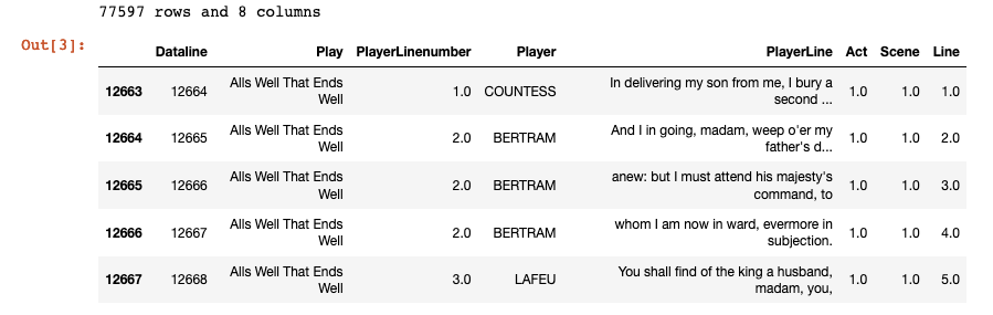
Thankfully, most of Shakespeare’s plays have been digitized. Using a Kaggle data-set we can download all 36 plays and load their scripts into a dataframe. Since scripts contain stage directions, which don’t give information about how characters relate to one another, we’ll drop those rows. Since we won’t be analyzing Shakespeare's histories we can also drop those.

import pandas as pd

plays_df = pd.read_csv("Shakespeare_data.csv")
# Drop stage directions (where there isn't an act/scene/line)
plays_df = plays_df[pd.notna(plays_df['ActSceneLine'])]
plays_df[['Act','Scene','Line']] = plays_df['ActSceneLine'].str.split('.',expand= True).astype(float)
plays_df = plays_df.drop('ActSceneLine',axis=1)

# Drop Shakespeare's histories
histories = ["King John", "Henry Iv", "Henry Vi Part 1", "Henry V",
            "Henry Vi Part 2", "Henry Vi Part 3", "Henry Viii",
            "Richard Ii", "Richard Iii"]
plays_df = plays_df[~plays_df["Play"].isin(histories)]

print("{} rows and {} columns".format(*plays_df.shape))
plays_df.head()

Now that the data is in a usable format we can start building our networks (one for each play). Since we’re interested in how characters relate to each other we’ll add a link, also called an edge, between two characters if they speak in the same scene. Characters that speak together frequently are probably connected in some meaningful way. This will form the basis for our network-first classification model.

Let’s use Shakespeare’s 1623 play All’s Well That Ends Well as an example. First we’ll isolate for that play’s dialogue. Then we’ll calculate how many times each character speaks, and keep those who meaningfully contribute to the structure of the play (those that speak more than 5 times).

play_name = "Alls Well That Ends Well"

single_play = plays_df[(plays_df['Play'] == play_name)]

# Group the df by character to get how often each speak
characters = single_play.groupby(['Player']).size().reset_index()
characters.rename(columns = {0: 'Count'}, inplace = True)
# Get top 20 characters
characters = characters[characters["Count"] > 5]

Next we’ll create the network. We can do this by going scene by scene and adding a link between two characters if they speak in the same scene. The more times those characters speak together in different scenes, the stronger their link will be.

from itertools import combinations
from networkx import write_gpickle as write_g
import networkx as nx

play_graph = nx.Graph()
play_graph.add_nodes_from(top_characters["Player"])

# Group by Act/Scene and count how often each character spoke per scene 
scenes_df = single_play.groupby(['Act','Scene','Player']).size()
scenes_df = scenes_df[scenes_df["Player"].isin(characters["Player"])]
scenes_df.rename(columns = {0: 'Count'}, inplace = True)

# Go scene by scene
for (act,scene), counts in scenes_df.groupby(['Act','Scene']):
    # Get all the characters that are in that scene
    characters = counts["Player"].tolist()
    # If a scene contains characters [A,B,C] we want our graph to
    # contain the edges [(A,B),(A,C),(B,C)]
    pairs = list(combinations(characters,2))
    for (a_char, b_char) in pairs:
        if character_graph.has_edge(a_char, b_char):
            play_graph[a_char][b_char]['weight'] += 1
        else:
            play_graph.add_edge(a_char, b_char,weight=1)

write_g(play_graph, "./graphs/{}.gpickle".format(play_name))

Repeat for all 27 plays, visualize, and these are the resulting networks! Now we need a way to distinguish between comedies and tragedies that only uses these networks.

How to Compare Networks

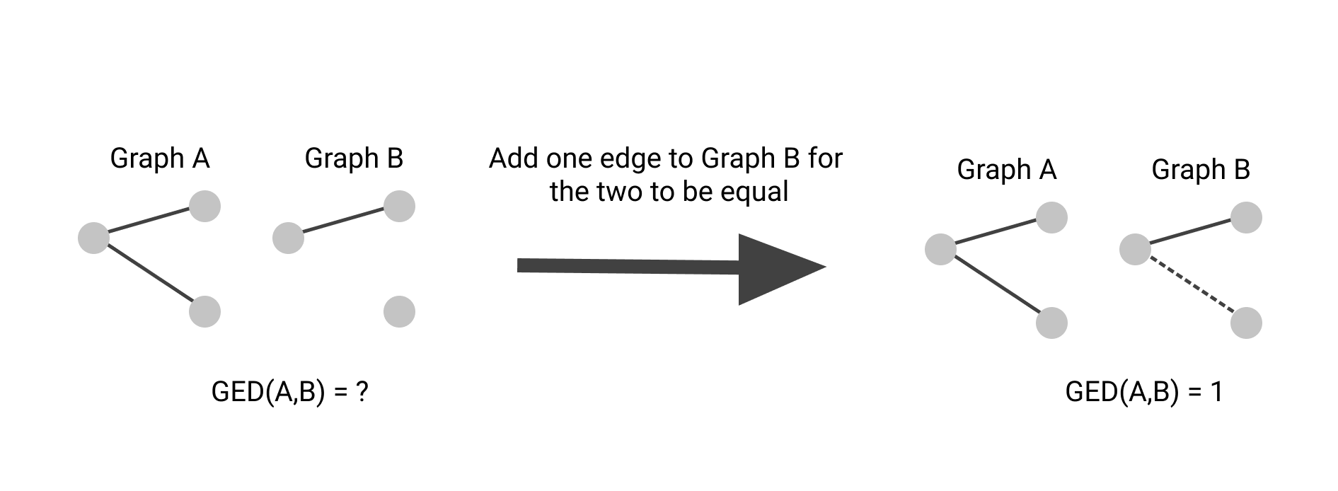The traditional way to compare networks.

Now that we’ve built networks for Shakespeare’s plays we need some way of distinguishing them. Unfortunately, there isn’t some straightforward way of comparing the structure of two networks. Traditionally, the most dominant method of comparison was called graph edit distance (GED). This method calculates how many edges would need to be reassigned between the two networks before they became identical. This is visualized in the image above. Unfortunately, this relies on each graph having the same number of nodes — or else they’d never be identical. Since our plays have a varied number of characters, we’ll need to turn to something else. GED is also relatively simple, and rarely captures the underlying structure of a network, so a more nuanced comparison method is needed.

Two graphs with similar structures despite different densities. Source.

To solve this, we turn to a 2018 paper published in the International Conference on Knowledge Discovery & Data Mining. These researchers define that two graphs are similar if information would flow through them in similar ways over time¹. The resulting method is called a Network Laplacian Spectral Descriptor, or NetLSD for short. They’re assumption is that information flows through a network similar to how heat diffuses throughout your air ducts. If each node in your network gives off some of its “heat” over time and passes it along the edges to its neighbors, then over time it will produce a signature that captures the network’s structure. So at each time step, all you have to do is sum up the amount of “heat” in the network. This is represented by h(t) and is visualized as the y-axis in the image below. Since each heat trace signature uses the same number of time steps, it’s much easier to compare networks of different sizes. By using this technique they were able to identify between different types of proteins and enzymes with a high level of accuracy (94–95%)¹.

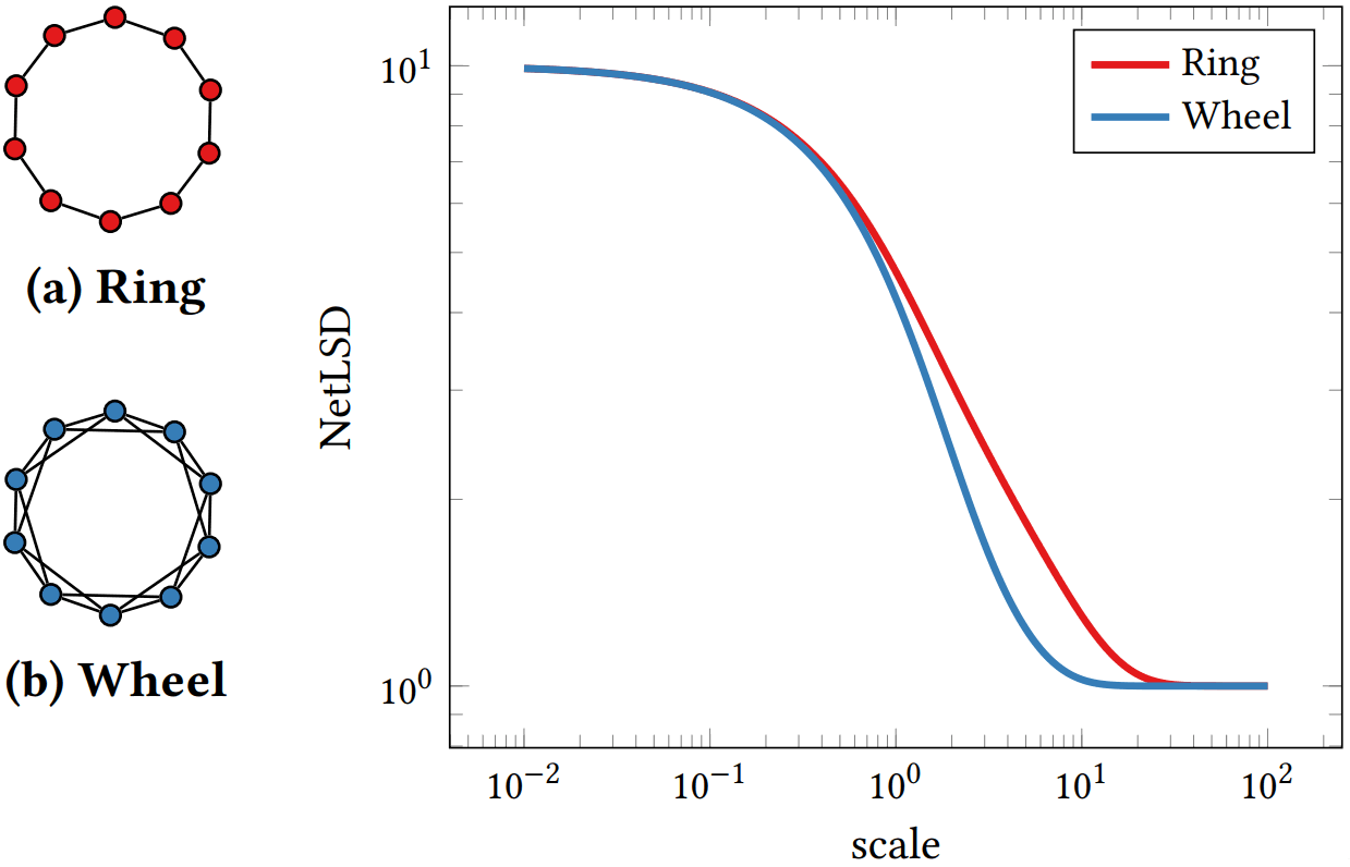NetLSD Heat signatures for two similar graphs: Source: Tsitsulin et al.

While implementing NetLSD is relatively simple (especially if you use their Python package) it does requires some background knowledge in how computers represent networks and linear algebra. For those who are interested here’s the original paper. Since NetLSD’s inner workings aren’t crucial to our task of classifying comedies and tragedies, I’ll move along.

Putting Everything Together

Now that we have a way of comparing networks in a meaningful way we can classify different plays. First, we’ll split the 27 plays up into two buckets: our training data, observed plays where we know the genre, and testing data, unknown plays that will be classified. We’ll use our knowledge of the previously observed plays to help classify the unknown ones. Since there are so few plays, I’ll reserve a third of the plays as testing data to validate the model.

from sklearn.model_selection import train_test_split
from numpy import concatenate as concat

com = [“A Midsummer Nights Dream”, “A Comedy Of Errors”,
        “Taming Of The Shrew”,“Two Gentlemen Of Verona”,
        “Loves Labours Lost”, “The Tempest”,“A Winters Tale”,
        “Cymbeline”, “Pericles”,”Alls Well That Ends Well”,
        “Measure For Measure”, “Troilus And Cressida”,
        “Twelfth Night”,“As You Like It”,
        “Much Ado About Nothing”, “Merchant Of Venice”,
        “Merry Wives Of Windsor”]

trag = [“Macbeth”,”Titus Andronicus”, “Romeo And Juliet”,
        “King Lear”,“Hamlet”,”Othello”, “Julius Caesar”,
        “Antony And Cleopatra”, “Coriolanus”, “Timon Of Athens”]

data = np.array(com+trag)

# Labels are what we're trying to predict (comedy or tragedy) 
labels = concat([np.full(len(com), “c”),np.full(len(trag), “t”)])

priors, test_data, prior_labels, test_labels = train_test_split(data, labels, test_size=0.33)

Next we’ll take all of our training data, the plays where we know the genre, and calculate their heat trace signatures.

import netlsd
from networkx import read_gpickle as read_g 

args = { "timescales": np.logspace(-2, 2, 250), "normalization": "empty" }

get_sig = lambda title: netlsd.heat(read_g("./graphs/{}.gpickle".format(title)),**args)

prior_sigs =[get_sig(title) for title in priors]

Let’s see if there’s a noticeable difference in how heat flows through a comedy vs a tragedy. It’s a little muddled, but it seems like tragedies retain more “heat” than comedies on average. Using these signatures we can start classifying the unknown plays.

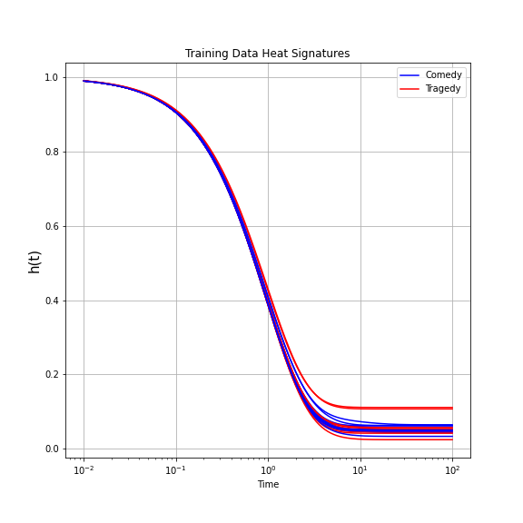Heat signatures for the prior observed plays (aka ‘training data’)

The process for classifying a new play is relatively simple. We calculate the unobserved play’s heat trace signature, and then find the five prior observed plays with the closest heat trace signatures. If the majority of those five are comedies then we label that play as a comedy, otherwise we label it as a tragedy. This is what’s called a k-nearest neighbor (KNN) classifier. KNNs don’t really model anything per say — which is why I prefer the term priors to training data — but with so few plays to work with a KNN is a reasonable choice.

from netlsd import compare as l2_distance

def knn_predict(title, prior_sigs, prior_labels,k=5):
    graph_sig = get_sig(title)
    distances = [l2_distance(graph_sig,ps) for ps in prior_sigs]
    total = pd.DataFrame({"ptype": prior_labels, "dist": distances})
    total = total.sort_values("Distance From Input")
    return total["ptype"].head(k).mode()[0]

pred = [knn_predict(play,prior_sigs,prior_labels) for play in data_test]

So how’d we do? Well, we were able to correctly classify 7 of the 9 plays in our testing data for a raw accuracy of 77.8%. The testing set contained 7 comedies and 2 tragedies, and we were able to correctly classify all of the tragedies and 5/7 comedies. This shows that comedies and tragedies produce distinct enough structures that we can tell which is which by only looking at the networks.

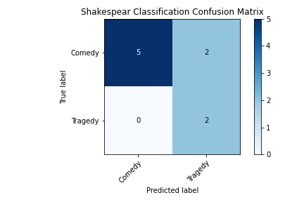Comedy/tragedy classification confusion matrix.

So What?

While 27 plays is a small sample, I’d argue that the principles of this experiment are sound. A network first approach lets us do something that, at first glance, seem pretty unlikely: we are able to figure out the genre of a play without looking at a single piece of dialogue. Personally, I think that is pretty cool.

So are you saying this means we don’t care about NLP anymore?

Obviously not. There’s a ton of rich information in language that’s lost when something like a play is abstracted into a network. However, networks give researchers flexibility to not rely on, or be bound by, language. This goes back to the example of comparing plays in different languages or from different time periods. And the applications don’t stop at comparing plays or movies. Disinformation is often spread en-mass by creating networks of social media bots that retweet and amplify each others fake news to give the illusion of legitimacy. Rather than focusing on what an account is saying, it could be more helpful to see if it’s connection network is similar to networks of disinformation bots that have been taken down. There are plenty of potential applications because networks are so malleable and can be used to represent almost anything. If you want to learn more about network science/graph theory and it’s applications, check out my website below! It has links to all my work.

[1]: Tsitsulin, Anton, Davide Mottin, Panagiotis Karras, Alexander Bronstein, and Emmanuel Müller. “Netlsd: hearing the shape of a graph.” In Proceedings of the 24th ACM SIGKDD International Conference on Knowledge Discovery & Data Mining, pp. 2347–2356. 2018.